Published online: 26.05.2019
Author: James M. Byrne

When I first started learning how to fit Mössbauer data, I blindly placed my trust in the fitting software, adding doublets and sextets whenever they seemed appropriate. However, I never stopped to think about what really makes up these specific line shapes. It took several years before I eventually decided to see if I could make more sense of these mysterious curves by drawing my own doublets and sextets in Excel. It turned out after a short period of troubleshooting that these lines were much easier to understand than I had first thought and I quickly realised it was even possible to fit them to raw data, first by guess work and then by using the solving tools in Excel. I now incorporate this strategy into my lectures because I think it provides students with a much better appreciation for the interpretation of the spectra when they can understand the fundamentals behind how the fitting actually works. The purpose of this page is to replicate this and provide a step by step guide to the fundamental aspects of data fitting.

Hopefully you already have heard a little bit about the theory of Mössbauer spectroscopy, so I will simply jump straight ahead and remind you of the fact that the characteristic Mössbauer spectrum is best described by a Lorentzian lineshape:

$$L(x) = I*{1\over \pi}{w/2 \over (x-x_0)^2+(w/2)^2}$$ Where \(I=\)intensity, \(x=\)velocity [mm/s], \(x_0 =\) centre of the curve, \(w =\) half width at half maximum

Based on just this simple equation, it is possible to create the classic singlets, doublets and sextets you should already be familiar with.

Creating a singlet

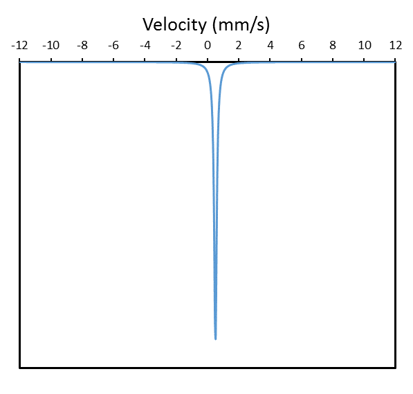
A good place to start is the singlet as it is the easiest and fastest type of lineshape you can create. If we create a figure using equation 1, you will see that x₀ simply describes the center shift parameter. Let's see what I mean:

1. Start a new Excel project
2. Make a column for velocity (this will be our x) with values from -12 to 12. The step size between each cell should be 0.047. We use this value because it is the velocity range, divided by the number of channels in the detector which is typically 512, i.e. (12- -12)/512=0.047
3. Make a column L using equation (1)
4. Make an absolute cell for I = 1
5. Make an absolute cell for w = 0.097 [mm/s]
6. Make an absolute cell for x0 = 0 [mm/s]
7. Plot a graph of velocity vs. L

When you plot the graph, you should see a peak, but most Mössbauer data is inverted (i.e. you see a dip rather than a peak). To correct for this, simply multiply all the values in your L column by -1. You should hopefully see a characteristic Mössbauer spectrum which looks like a singlet.

Now change the value of x0 and see what happens. This value of x0 clearly corresponds to the center shift.

Download workbook - Singlet

Creating a doublet

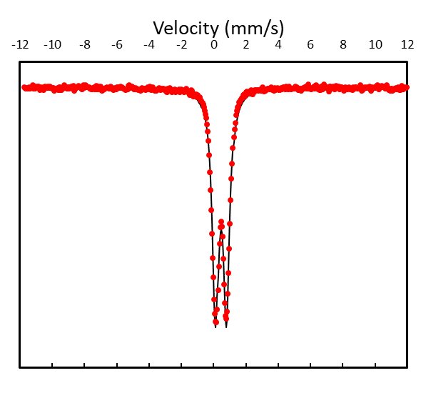
A singlet is nice and easy, but with the exception on of a few examples, most environmental samples have spectra which are characterised by doublets or sextets. Can you think how to change the Lorentzian equation so that we can plot a doublet? All you have to do is to plot two of them and add them together. So we can simply adjust the equation describing L(x) and introduce a left and right side.

$$L(x) = L(x)_L+L(x)_R=I*{1\over \pi}{w/2 \over (x-x_L)^2+(w/2)^2}+I*{1\over \pi}{w/2 \over (x-x_R)^2+(w/2)^2}$$ Where \(I=\)intensity, \(x=\)velocity [mm/s], \(x_0 =\) centre of the curve, \(w =\) half width at half maximum

Here you should notice that I have changed x₀ to x_L and x_R for the left and right Lorentzians respectively. These terms now contain information that correspond to both center shift (CS) and quadrupole splitting (QS) parameters:

$$x_L = CS-{QS\over 2}$$ $$x_R = CS+{QS\over 2}$$

This means we can rewrite equation (2), and factor out the intensity (I) of the curve :

$$L(x) =I*\Bigg({{1\over \pi}{w/2 \over (x-CS-{QS\over 2})^2+(w/2)^2}+{1\over \pi}{w/2 \over (x-CS+{QS\over 2})^2+(w/2)^2}}\Bigg)$$

So let's try and plot this: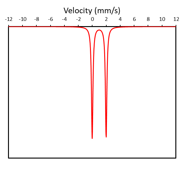

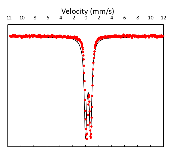
1. Start a new Excel project
2. Make a column for velocity (this will be our x) with values from -12 to 12. The step size between each cell should be 0.047. We use this value because it is the velocity range, divided by the number of channels in the detector which is typically 512, i.e. (12- -12)/512=0.047
3. Make an absolute cell for I = 1
4. Make an absolute cell for w = 0.097 [mm/s]
5. Make an absolute cell for CS = 0 [mm/s]
6. Make an absolute cell for QS = 0 [mm/s]
7. Make a column L using equation (5)
8. Plot a graph of velocity vs. L

You will probably only see one peak! This is because the hyperfine parameters of each Lorentzian are set to 0. Change one or both of CS or QS and you will see the peak split into two distinct peaks and shift along the velocity axis. You can also change the value of w to see both halves of the spectrum become broader or narrower (be careful, 0.097 is the theoretical minimum).

Download workbook - Doublet

Working with data

Now we have a very basic spectrum, but how can we use this to fit our data? First, we need to get some data. Either you have your own, or we can just work with some that already exists. Download the spectrum below:

Unknown 1

This is just a basic spectrum which can be described by a doublet. Follow the steps below to get started:

1. Start a new Excel project
2. Import your data into two separate columns and give them the headings "Velocity" and "Data".
3. Create a new column with the heading "Fit".
4. Make an absolute cell for I = 3E5 (this value should be changed accordingly if you imported your own data)
5. Make an absolute cell for background (Bkgd) = 8.65E6 (this cell is now required because your data will always have a background intensity which you will need to account for. If you imported your own data, you should change this value accordingly)
6. Make an absolute cell for w = 0.097 [mm/s]
7. Make an absolute cell for CS = 0 [mm/s]
8. Make an absolute cell for QS = 0 [mm/s]
9. In the "Fit" column, fill the cells with equation (5), however use the "Velocity" column from the imported data as your x.
10. Plot a graph which shows both the "Fit" and "Data" against "Velocity"
11. Manually change CS and QS so that your spectrum closely fits the data. You might also need to change the values for intensity (I), background and linewidth (w). Suggested parameters include CS = 0.35, QS = 0.77, w = 0.5.

You have now completed a very basic and crude way of fitting your Moessbauer data. This is of course not very scientific and we need a more robust method to analyse our data. There are many different approaches to doing this, but one common method is to use a regression based analysis where the difference between the "data" and the "fit" is minimized.

In your workbook, add a new column with the heading "least squares". Fill the cells in this column with (fit-data)^2. Now create a new cell which sums all of the values in the least squares column, i.e.:

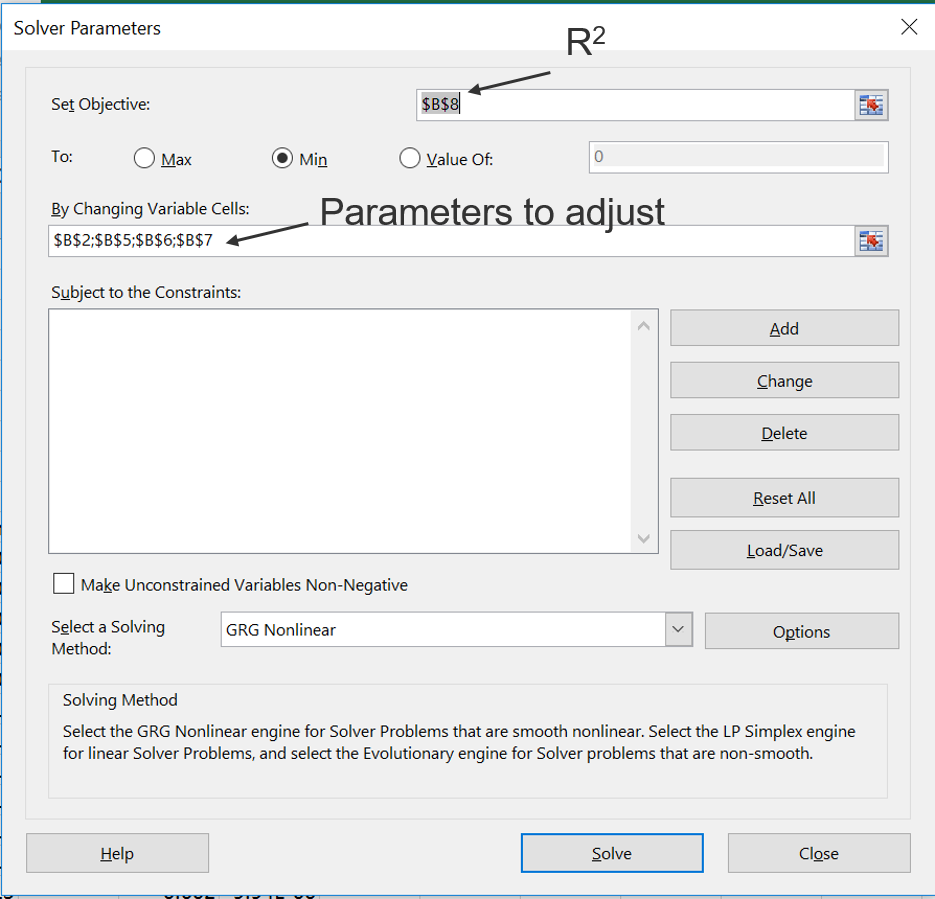
$$R^2 = {\Sigma{(fit-data)}^2}$$

The general goal is to minimize R², so try and adjust your hyperfine parameters again so that it is even lower. Normally, your fitting software will just try minimize this number by changing the hyperfine parameters. There is a method for doing this in Excel using a plugin called Solver. To install in Excel:

1. Go to File > Options > Add-ins
2. Press Go
3. Tick "Analysis ToolPak" and "Solver Add-in"
4. Press OK and then restart Excel
5. Solver should now be installed under "Data" ribbon.
6. Select the cell containing the sum of your least squares (i.e. R² and press "Solver".
7. The Set Objective field should contain the cell describing R².
8. We want to minimize R² so select the "Min" radio button
9. Select all the hyperfine parameters (CS, QS, I, Bkg and w) in "By Changing Variable Cells".
10. Press Solve at the bottom.

You have now made a very basic fitting program in which the hyperfine parameters should be able to describe the mystery sample (Figure 5). The sample was measured at room temperature. Look up the center shift and quadrupole splitting on the Mosstool database and try to determine the mineral identity.

Download workbook - Doublet with real data

Creating a sextet

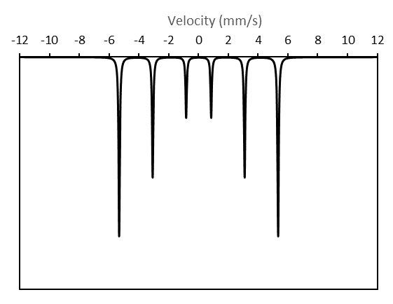
Now we will move onto the sextet, which is commonly observed when analysing crystalline iron oxides such as hematite, goethite or magnetite, or paramagnetic mineral phases below their blocking temperature. How do we create a sextet? We just need to add six Lorentzians together:

$$L(x) = L(x)_1+L(x)_2+L(x)_3+L(x)_4+L(x)_5+L(x)_6$$

I have not written out the details for each of the individual Lorentzians because it would be far too long here. However, in general we need to replace the x₀ for each individual Lorentzian as follows:

\(Lorenzian\)	$$x_0$$
\(1\)	$$0-(Bhf/B_c*D3/2)+IS+QS$$
\(2\)	$$0-(Bhf/B_c*D2/2)+IS-QS$$
\(3\)	$$0-(Bhf/B_c*D1/2)+IS-QS$$
\(4\)	$$0+(Bhf/B_c*D1/2)+IS-QS$$
\(5\)	$$0+(Bhf/B_c*D2/2)+IS-QS$$
\(6\)	$$0+(Bhf/B_c*D3/2)+IS+QS$$

Where \(B_c=32.95, D1 = 1.679, D2 = 6.1525\) and \(D3 = 10.625\).

You might notice that the above equation does not account for differences in the intensities of the individual peaks of a sextet. In general, these often follow the ratio of 3:2:1:1:2:3 for peaks 1-6 respectively. Therefore, lets update our equation to include these ratios:

$$L(x) = 3L(x)_1+2L(x)_2+L(x)_3+L(x)_4+2L(x)_5+3L(x)_6$$

Now we are ready to create a sextet:

1. Start a new Excel project
2. Make a column for velocity (this will be our x) with values from -12 to 12. The step size between each cell should be 0.047. We use this value because it is the velocity range, divided by the number of channels in the detector which is typically 512, i.e. (12- -12)/512=0.047
3. Make an absolute cell for I = 1
4. Make an absolute cell for w = 0.097 [mm/s]
5. Make an absolute cell for CS = 0 [mm/s]
6. Make an absolute cell for QS = 0 [mm/s]
7. Make an absolute cell for Bhf = 33 [mm/s]
8. I now recommend making six columns for each of the terms within the equation for L(x). This will make it easier to handle in Excel.
9. Add a seventh column with the title "Fit" which is simply the sum of each of the six individual columns created in step 7.
10. Plot a graph of Velocity vs. Fit

Download workbook - Sextet

Working with data

Now we have a very basic spectrum for a sextet, but how can we use this to fit our data? First, we need to get some data. Either you have your own, or we can just work with some that already exists. Download the spectrum below:

Unknown 2

I now challenge you to try and fit the data using the same approach described for the doublet. The principle is almost identical and through the use of the Solver function, you will be able to determine the identify of Unknown 2. If you get stuck, download the fully worked solution:

Download workbook - Sextet with real data

Remarks

I hope that this brief tutorial has given you at least a very basic understanding of how Moessbauer data fitting works. There are of course much more complicated models which can be used, but the basic principles remain the same. Happy fitting!