To measure a Mössbauer spectrum, the source is mounted on a motor and is moved to Doppler shift from small to large energies. As the source moves through both positive and negative Doppler velocities, the spectra must be folded prior to fitting in Recoil.
The folded data must also be calibrated to correct for differences between the matrix of the source and the sample. We use metallic α-Fe for this and the calibration file defines a CS of 0 and Lorentzian line broadening.
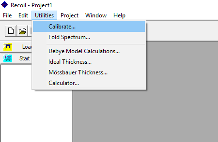
Calibration
Open Recoil and click 'Start new project'. The help function unfortunately no longer works in this version of the software although the manual and some helpful articles are available with the software.
Select 'Utilities' then 'calibrate' and select 'all files' as file type. Choose the file 'cal v6.txt' (we have a separate calibration file for each measurement velocity).
Figure 1
Select the option 'Automatically accept the peaks fitted by the computer' and click next.
Ensure the options 'alpha-Fe' and 'constant acceleration' are selected and click next. You may get an error message about deviation at this point but it is mostly fine to ignore it.
Click finish and save the new calibration file as a .cal.
Note: one must also fit the inner doublets of the calibration file itself to determine the correct Lorenztian half width at half maximum, which is used for the peak shapes during the fitting procedure.
Folding
Again, select 'Utilities' then 'fold spectrum' and select 'all files' as file type. Choose the file '150616_NAu1_13K_v6.txt'.
Select the calibration file you made in the previous section. You will be asked if you wish to apply a cubic spline correction, click no.
The folded spectrum will appear in the main window. Save the folded spectrum (file - save as).
Fitting Mössbauer spectra
- Doublets (QSD sites)
We are now ready to fit the spectrum that we have folded. The spectrum is a sample of nontronite, NAu-1, that has been partially reduced and contains an amount of structural Fe(II), measured at 13 K. Our aim is to determine the % Fe(II)/Fe(total) ratio of the sample.
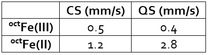
From prior knowledge of the sample (NAu-1 contains only octahedral Fe) and visual inspection of the spectra, we can expect to fit two doublets to the spectrum, for Fe(III) and Fe(II) respectively. The anticipated parameters for these Fe sites are provided in the table below.
Table 1 - Hyperfine parameters of partially redued nontronite (NAu-1). CS - center shift; QS - quadrupole splitting.
Click 'Start New Analysis' and then select VBF Site Analysis (Voigt Based Fitting). Recoil also allows for the use of other fitting regimes, as required.
Figure 2
Select the folded spectra you previously saved.
Save this as a .vbf file (file - save as).
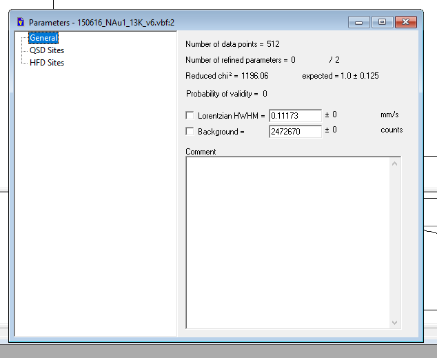
You will see three options in the left hand column. General, QSD (for fitting singlet and doublet sites) and HFD (for fitting hyperfine field parameters for sextet sites). Check that you are in the 'general' menu to begin with.
Insert the value for Lorentzian HWHM as calculated for your calibration file (see note in the calibration section). For the example here, this value is 0.136678.
Figure 3
Right click 'QSD Sites' and click 'add site'. Rename the new site that appears on your menu 'Fe(III)1' by clicking on the text to select it.
Figure 4
Type in the value suggested for Centre Shift (CS) from the above Table into the delta0 box and press enter. Note how the position of the peak moves from 0 to 0.5. You can adjust the range of the x-axis by clicking on it. Save the fit: it is good practice to regularly save your fits so if you mess up you can reload an earlier version!
Select 'Analysis' and then 'Fit spectrum'. Select 'use the covariance matrix of the fit' and press ok. The software will then iteratively fit the parameters that you have checked. As we are currently only fitting CS and area, the software will attempt to fit a singlet to the spectra. As we are expecting a doublet, we must also include quadrupole splitting (QS) parameters.
Add in the anticipated value for QS from the table in the 'component 1' menu, save the fit and then fit the spectrum again. You will observe a fit that appears to be in the correct position, but with sharper peaks than those of the spectra. To adjust the broadness of the peaks, try adjusting the 'sigma' parameter to approximately 0.3 and fit again. This adds further Lorentzian peaks to the VBF to adjust the peak shape.
Figure 5
Once you are happy with your fit for Fe(III), create a new site for Fe(II) and fit the Fe(II). It is advisable to uncheck your parameters for Fe(III) while you do this.
Once you are happy with your fit for Fe(II), you can begin to fit the Fe(III) and Fe(II) parameters together. To avoid over-fitting, it is advisable to begin with fitting single parameters together (e.g. CS) and to gradually include more parameters in the fit. It is not advisable to let the software fit until you have approximately fitted your chosen parameters by eye.
Figure 6
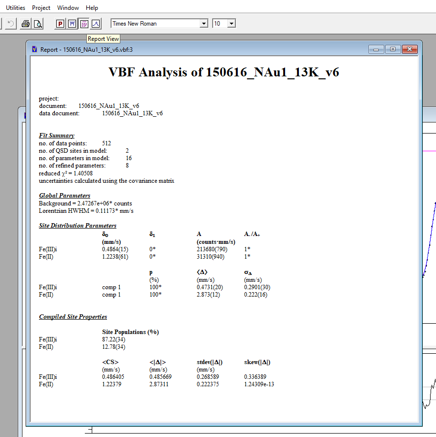
When your fit is finalised, you can access an overview of the fit parameters and error statistics by accessing the 'Report View' from the tool bar menu. Export this by saving it as a .rtf file, which can be opened in MS Word.
To export your data for plotting in an external graphing programme, select the 'Plot View' and save the data as a .fit file. This can then be imported into excel in the same way as a text file.
- Sextets (HFD sites)
The second example is a sample of an Fe oxide/oxyhydroxide precipitate (180323 KR 3mM 57Fe(II) + AQDS 4K v12, ensure you select the '4K sample'). Your task is to suggest the phases that are present.
Begin by folding the spectrum, note that as this was measured at a velocity of 12 mm/s you will have to create and use a v12 calibration file. The Lorenztian HWHM for this file is 0.159005.
Figure 7
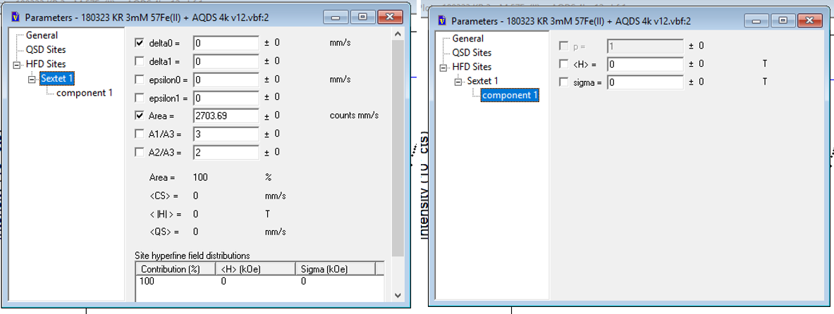
As the spectrum exhibits hyperfine splitting (sextets) then we must this time add HFD sites. In this menu delta0 refers to CS and epsilon0 QS/2 (Quadrupole shift). The units for the hyperfine splitting parameter, H, can be changed in the Edit - preferences menu.
Figure 8
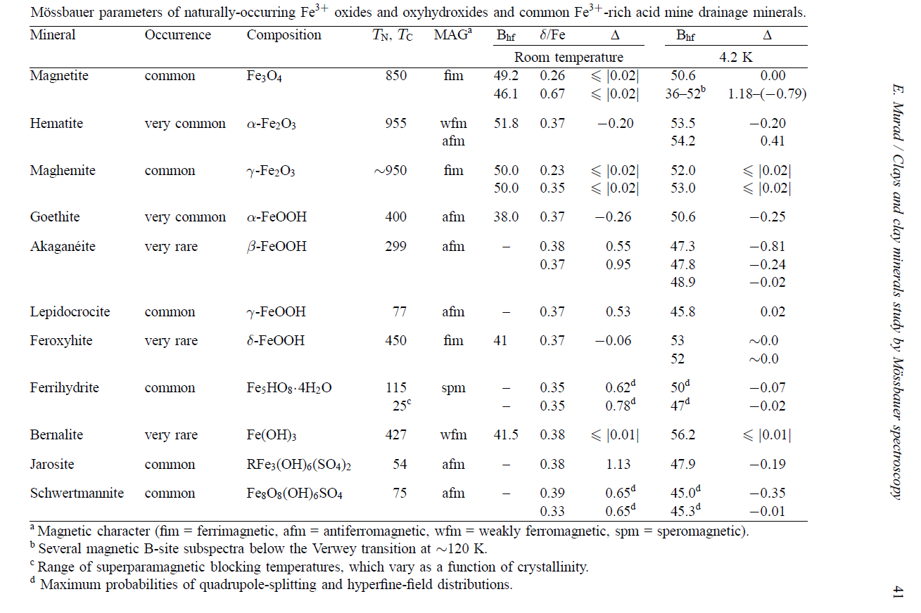
Fit two sextet Fe sites to the spectrum and then use Table 2 and Mosstool to suggest the composition of the sample.
Table 2
Quick Questions:
How else could we use Mössbauer to help identify the sample?
You will also find a copy of the same sample, this time measured at 77 K. Try and fit this. You will struggle to get a good fit at this temperature. Why do you think this is?
How much sample is required?
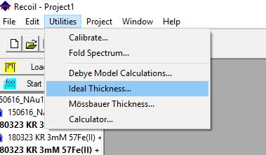
Recoil has a built in function to calculate the optimum amount of sample required based on sample stoichiometry.
Figure 9
You can access this through the 'Utilities - Ideal Thickness' menu and will then be asked to enter the stoichiometry of the sample and the width of the sample holder (in most cases this is 1.0 cm).
References
Murad, E., Clays and clay minerals: What can Mössbauer spectroscopy do to help understand them? Hyperfine Interactions, 1998. 117, 39-70.
Contact us
Did you like this tutorial? Is there anything which can be improved? Or perhaps you want to contribute you own tutorial? If so, please get in touch.